Exomoon Transit Modeling

import numpy as np
import matplotlib.pyplot as plt
import gefera as gf

Define the parameters of the transit:

t = np.linspace(-0.6, 0.2, 10000)

# dynamical parameters for the planet
ap = 215                    # semimajor axis in stellar radii
tp = -91.25                 # starting time in days
ep = 0.0                    # eccentricity
pp = 365                    # period in days
wp = 0.1 * np.pi / 180      # longitude of periastron in radians
ip = 89.8 * np.pi / 180     # inclination in radians

# dynamical parameters for the moon
am = 10                     # semimajor axis of moon's orbit around the planet
tm = -4.2                   # starting time in days
em = 0.0                    # eccentricity
pm = 8                      # period in days
om = 45 * np.pi / 180       # longitude of the ascending node in radians
wm = -90 * np.pi / 180      # longitude of periastron in radians
im = 90.0 * np.pi / 180     # inclination in radians
mm = 0.01                   # moon/planet mass ratio

# other parameters
u1 = 0.5                    # first quadratic limb-darkening parameter
u2 = 0.3                    # second quadratic limb-darkening parameter
rp = 0.1                    # radius of the planet in stellar radii
rm = 0.06                   # radius of the moon in stellar radii

Now we can build the system. We start by defining the primary orbit, or the orbit of the planet, using gf.orbits.PrimaryOrbit. We then define the orbit of the moon using gf.orbits.SatelliteOrbit. We pass both of these orbits to gf.systems.HierarchicalSystem to define the dynamical system.

po = gf.orbits.PrimaryOrbit(ap, tp, ep, pp, wp, ip)
mo = gf.orbits.SatelliteOrbit(am, tm, em, pm, om, wm, im, mm)
sys = gf.systems.HierarchicalSystem(po, mo)

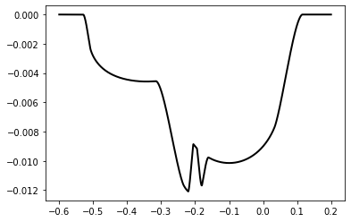
Now let’s compute the flux (and its gradients!) and plot it:

%time flux, grad_flux = sys.lightcurve(t, u1, u2, rp, rm, grad=True)
plt.plot(t, flux, color='k', linewidth=2)

CPU times: user 18.1 ms, sys: 9.05 ms, total: 27.2 ms
Wall time: 28.4 ms

[<matplotlib.lines.Line2D at 0x114e8b6a0>]

The gradients are stored in a dictionary keyed to the names of the parameters, which are given as a1, t1, e1... a2, t2, e2 rather than ap, tp, ep... am, tm, em to account for the fact that the bodies need not be a planet and moon (they could both be planets, or a star and a planet). Here we access them by repackaging them into a list and looping over them rather than through dictionary keys.

fig, axs = plt.subplots(6, 3, figsize=(15, 15))
axs = axs.flatten()

names = [
    r'$a_p$', r'$t_p$', r'$e_p$', r'$P_p$', r'$\omega_p$',
    r'$i_p$', r'$a_m$', r'$t_m$', r'$e_m$', r'$P_m$',
    r'$\Omega_m$', r'$\omega_m$', r'$i_m$', r'$M_m$',
    r'$r_p$', r'$r_m$', r'$c_1$', r'$c_2$'
]

for i, (name, g) in enumerate(list(grad_flux.items())):

    axs[i].plot(t, g, color='k', linewidth=2)
    axs[i].annotate(
        names[i],
        xy=(0.85, 0.75),
        xycoords='axes fraction',
        fontsize=20, bbox={'facecolor': 'w'}
    )

If we want to see what the transit we modeled actually looks like we can use the snapshots function to build a static movie of the transit:

times = t[::1000]
fig, axs = plt.subplots(1, len(times), figsize=(30, 3))
gf.animate.snapshots(sys, axs, times, rp, rm, ld_params=[u1, u2])